
|
|
|
Data Analytics using R -- mapping statistical data: part 1
The world of visual and geospatial analysis continues to morph and evolve. So it is with R's geospatial analysis evolvement. R (more about R) is an open source language and environment for statistical computing and graphics. R has many similarities with the Statistical Analysis System (SAS), but is free ... and widely used by an ever increasing user base. R is used throughout the ProximityOne Certificate in Data Analytics course. For now, in the areas of mapping and geospatial analysis, R is best used in a companion role with Geographic Information System (GIS) software like CV XE GIS. Maybe it will always be that way. R's features to 1) perform wide-ranging statistical analysis operations and 2) to process and manage shapefiles and relate those and other data to many, many types of data structures are among R's key strengths. Mapping with R The following Web-based interactive map has been developed totally using R. Aside from satellite imagery, which can be added, this application has the look and feel of a Google maps application. Yet the steps to develop the application are far different and much closer to more traditional GIS software and data structures .. and there are no proprietary constraints. Mapping with R is not a geospatial panacea. See these considerations & FAQs. Join us in weekly Data Analytics Lab sessions to learn about developing this type of mapping application and geospatial analysis. See more about this application in narrative below the map. Create & publish this interactive map or variation - details below R generates the final product HTML as shown above. This application illustrates use of a Census county TIGER/Line shapefile integrated with Census 2010 demographics. Participants in the ProximityOne Data Analytics course learn how to develop the types of maps using a range of TIGER/Line shapefiles (e.g., census blocks, metros, congressional districts, etc.). Integrate subject matter from the American Community Survey and many other Federal statistical programs. R and the ProximityOne CV XE GIS tools work together to expand the range of analytics to an unlimited set of possibilities. Create & Publish Above Web-Based Map Follow these steps to develop and publish the above map or variations (such as a different state). • Install R .. select Download R for Linux or Mac OS X or Windows (recommended) options at top of page. • Start R using desktop icon (use 64 is your machine offers 32 and 64) • Copy and paste *all* text the scroll section below (text only) to the control prompt in the R window; .. at pointer as shown in this graphic then press enter. .. processing starts immediately. • Be patient, watch the messages, wait for the HTML map to be generated and displayed. About 4 minutes. • After map displays, enter "q()" without quotes at R command prompt to quit; do not save workspace. • Join us in weekly Data Analytics Lab sessions to discuss operations & use. #the following 4 commands only need to be run once # ... in the event you run the remainder of the command multiple times install.packages('leafletR') install.packages('rgdal') install.packages('rgeos') install.packages('sp') library(leafletR) library(rgdal) #for reading/writing geo files library(rgeos) #for simplification library(sp) # large file; may take a few minutes to download url<-"http://www2.census.gov/geo/tiger/TIGER2010DP1/County_2010Census_DP1.zip" downloaddir<-"c:/Leaflet" destname<-"tiger.zip" download.file(url, destname) unzip(destname, exdir=downloaddir, junkpaths=TRUE) ###### filename<-list.files(downloaddir, pattern=".shp", full.names=FALSE) filename<-gsub(".shp", "", filename) # may take 1 minute to read dat<-readOGR(downloaddir, filename) # Create a subset of New York counties; 48 is the FIPS code for NY; # change 48 to 20 to make Kansas map. subdat<-dat[substring(dat$GEOID10, 1, 2) == "48",] subdat<-spTransform(subdat, CRS("+init=epsg:4326")) # assign pseudo names to field names names(subdat)[names(subdat) == "DP0010001"]<-"Population" names(subdat)[names(subdat) == "NAMELSAD10"]<-"County" # save required items (only 2 needed from broader set) subdat_data<-subdat@data[,c("County", "Population")] subdat<-gSimplify(subdat,tol=0.01, topologyPreserve=TRUE) subdat<-SpatialPolygonsDataFrame(subdat, data=subdat_data) # Start LeafletR operations # Create GeoJSON leafdat<-paste(downloaddir, "/", filename, ".geojson", sep="") writeOGR(subdat, leafdat, layer="", driver="GeoJSON") cuts<-round(quantile(subdat$Population, probs = seq(0, 1, 0.20), na.rm = FALSE), 0) cuts[1]<-0 # Fields to use in the map click popup popup<-c("County", "Population") # Gradulated legend based on an attribute (population field) sty<-styleGrad(prop="Population", breaks=cuts, right=FALSE, style.par="col", # style.val=rev(heat.colors(5)), leg="Population (2010)", lwd=1) style.val=c("#eff3ff","#bdd7e7","#6baed6","#3182bd","#08519c"), leg="Population 2010", fill.alpha=0.7, rad=8, alpha=1,lwd=2,col="#006400") # Create map and load into browser map<-leaflet(data=leafdat, dest=downloaddir, style=sty, title="index", base.map="osm", incl.data=TRUE, popup=popup) # view HTML source code and optionally copy/use in your own web page browseURL(map) Corresponding CV XE GIS Project & View The following graphic illustrates use of the same shapefile used in the R application with a variation on colors and other details. Follow the steps below the graphic to install and use this GIS project on your Windows computer. 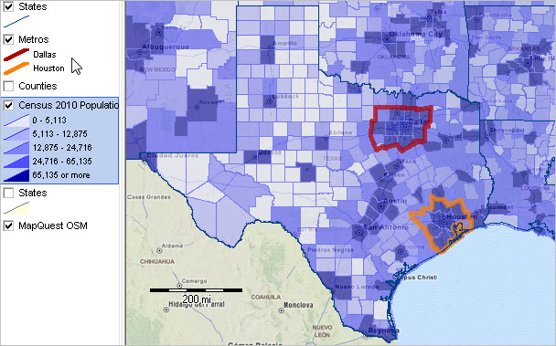 View developed using CV XE GIS and related GIS project. Census 2010 DPSF GIS Project/Datasets 1. Install the ProximityOne CV XE GIS ... omit this step if CV XE GIS software already installed. ... run the CV XE GIS installer ... take all defaults during installation 2. Download the Census 2010 DPSF GIS Project fileset ... requires ProximityOne User Group ID (join now) ... unzip Census 2010 DPSF GIS project files to new local folder c:\msd 3. Open the census2010_county_dpsf.gis project ... after completing the above steps, click File>Open>Dialog ... open the file named C:\msd\census2010_county_dpsf.gis 4. Done .. the start-up view is similar to the graphic above. Join us in weekly Data Analytics Lab sessions to discuss operations & use. Mapping with R -- Considerations & FAQs Each of us comes to this section with different experiences and skill sets. It is easy to be tripped up due to some minor detail .. right down to a missing, additional, misplaced or incorrect single character. The following are notes about using the text (command list) in the scroll section above. 1. Installing R packages There are many "packages" that may be installed to use R for various applications. Unless otherwise described, only Theses packages are installed after completing R installation and must be installed using R. Only 4 packages are needed to develop the objective map. The 4 command lines at the top of the scroll section only need to be run once; loading them into your personal library. In getting started, take the defaults.
# ... in the event you run the remainder of the command multiple times
install.packages('leafletR') install.packages('rgdal') install.packages('rgeos') install.packages('sp') 2. Repeated use of the script (command line set) After running the script once, you may want to experiment with variations and copy the relevant command lines to a reusable text file. Omit the 4 install package lines. 3. Being patient for some operations Some steps require more processing time than others. Wait for completion unless you see an error message. 4. Create & publish a different state? See the code section as shown here:
# Create a subset of New York counties; 48 is the FIPS code for NY;
To run Kansas, the modified line would be structured as follows:# change 48 to 20 to make Kansas map. subdat<-dat[substring(dat$GEOID10, 1, 2) == "48",] subdat<-dat[substring(dat$GEOID10, 1, 2) == "20",] Substitute the state FIPS code for 48 (the Texas FIPS code) to run any state. ProximityOne User Group Join the ProximityOne User Group to keep up-to-date with new developments relating to metros and component geography decision-making information resources. Receive updates and access to tools and resources available only to members. Use this form to join the User Group. Support Using these Resources Learn more about accessing and using demographic-economic data and related analytical tools. Join us in a Data Analytics Lab session. There is no fee for these one-hour Web sessions. Each informal session is focused on a specific topic. The open structure also provides for Q&A and discussion of application issues of interest to participants. Additional Information ProximityOne develops geodemographic-economic data and analytical tools and helps organizations knit together and use diverse data in a decision-making and analytical framework. We develop custom demographic/economic estimates and projections, develop geographic and geocoded address files, and assist with impact and geospatial analyses. Wide-ranging organizations use our tools (software, data, methodologies) to analyze their own data integrated with other data. Follow ProximityOne on Twitter at www.twitter.com/proximityone. Contact us (888-364-7656) with questions about data covered in this section or to discuss custom estimates, projections or analyses for your areas of interest. |
|
|