|
|
|
-- tools to build and use geographic relationship files Which census blocks or block groups intersect with one or a set of school attendance zones (SAZ)? How to determine which counties are touched by a metropolitan area? Which are contained within a metropolitan area? Which pipelines having selected attributes pass through water in a designated geographic extent? This section reviews use of the ProximityOne Shp2Shp tool and methods to develop a geographic relationship file by relating any two separate otherwise unrelated shapefiles. Try it yourself ... see details below. • Relating 115th Congressional Districts and Census Blocks; see below • Relating School Attendance Zones & Census Blocks; see below As an example, use Shp2Shp to view/determine block groups intersecting with custom defined study/market/service area(s) ... the only practical method of obtaining these codes for demographic-economic analysis. 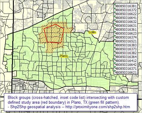 - the custom defined polygon was created using the CV XE GIS AddShapes tool. Many geodemographic analyses require knowing how geographic objects (points, lines, polygons) geospatially relate to others. Examples include congressional/legislative redistricting (see census block/congressional district example below), sales/service territory management and school district attendance zones. The CV XE GIS Shape-to-Shape (Shp2Shp) relational analysis feature provides many geospatial processing operations useful to meet these needs. Shp2Shp determines geographic/spatial relationships of shapes in two shapefiles and provides information to the user about these relationships. Shp2Shp uses the DE-9IM topological model and provides an extended array of geographic and subject matter for the spatially related geometries. Sh2Shp helps users extend visual analysis of geographically based subject matter. Examples: • county(s) that touch (are adjacent to) a specified county. • block groups(s) that touch (are adjacent to) a specified block group. • census blocks corresponding to a specified school attendance zone. • attributes of block groups crossed by a delivery route. Block Groups that Touch a Selected Block Group The following graphic illustrates the results of using the Shp2Shp tool to determine which block groups touch block group 48-85-030530-2 -- a block group located within McKinney, TX. Shp2Shp determines which block groups touch this block group, then selects/depicts (crosshatch pattern) these block groups in the corresponding GIS map view. 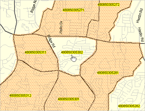
Geographic Reference File In the process, Shp2Shp creates a geographic relationship file as illustrated below. There are six block groups touching the specified block group. As shown in the above view, one of these block groups touches only at one point. The table below (derived from the XLS file output by Shp2Shp) shows six rows corresponding to the six touching block groups. The table contains two columns; column one corresponds to the field GEOID from Layer 1 (the output field as specified in edit box 1.2 in above graphic) and column 2 corresponds to the field GEOID from Layer 2 (the output field as specified in edit box 2.2 in above graphic). The Layer 1 column has a constant value because a query was set (geoid='480850305302') as shown in edit box 1.3. in the above graphic. Any field in the layer dataset could have been chosen. The GEOID may be used more often for subsequent steps using the GRF and further described below. It is coincidental that both layers/shapefiles have the field named "GEOID".
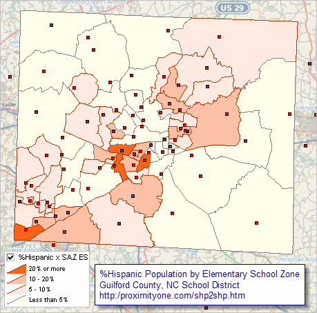
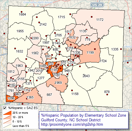
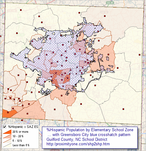
Note that in the above example, only the geocodes are output for each geography/shape meeting the type of geospatial relationship. Any field within either shapefile may be selected for output (e.g., name, demographic-economic field value, etc.) How it Works -- Shp2Shp Operations The following graphic shows the settings used to develop the map view shown above. 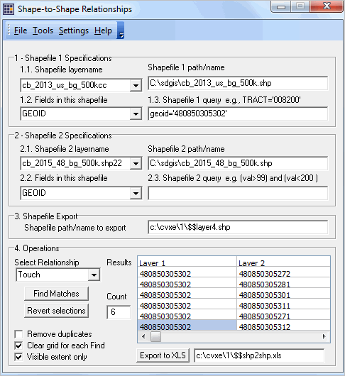 Review of basic steps to use Shp2Shp • Shp2Shp operates on the GIS project in use. • If a Web Tiles layer (e.g. "Base Layer" or "Open Streets Map" is in use, remove that layer .. do not save/resave the project With CVXE running, start Shp2Shp from the main menu File>Tools>Shp2Shp. The above form appears. • Select the first layer using the 1.1. dropdown. This shows all available layers in the GIS project. • Select the field from layer 1 to be used in the GRF using the 1.2. dropdown. • Optionally set a filter/query to be applied to Layer 1 in the 1.3. edit box. • Select the second layer using the 2.1. dropdown. This shows all available layers in the GIS project. • Select the field from layer 2 to be used in the GRF using the 2.2. dropdown. • Optionally set a filter/query to be applied to Layer 2 in the 2.3. edit box. • Select the type of geographic relationship. • In the simplest situation, click the Find Matches button. .. processing starts. .. when complete the results grid is displayed (see example in above graphic • After grid displays, optionally click Export button to save the grid to the designated XLS file. • Repeat the process as desired. Geographic Relationships Supported The Select Relationships dropdown shown in the above graphic is used to determine what type of spatial relationship is to be used. Options include: • Equality • Disjoint • Intersect • Touch • Overlap • Cross • Within • Contains See more about the DE-9IM topological model used by Shp2Shp. Try it Yourself • Use any version of CV XE GIS (March 14, 2017 or more recent-- see date in Help>About) .. not yet installed? Register for no fee installer (Windows). • Use the unmodified default start-up project c:\cvxe\1\cvgis.gis. • Start CV XE GIS. • Delete the layer named "Base Layer". Do not save or resave the project • Using Main Menu (top toolbar), select File>Tools>Shp2Shp. The start-up view of the form shown below appears. Shp2Shp Operations The following graphic shows the settings used to develop the map views shown below. • Select the first layer using the 1.1. dropdown as "CBSAs TX". • Select the field from layer 1 to be used in the GRF using the 1.2. dropdown. .. Use "GEOID". • Optionally set a filter/query to be applied to Layer 1 in the 1.3. edit box. .. key in the value "geoid='19100'" (no quotation marks, but leave apostrophe marks; .. this says to use only CBSA 19100 -- Dallas. • Select the second layer using the 2.1. dropdown. This shows all available layers in the GIS project. • Select the field from layer 2 to be used in the GRF using the 2.2. dropdown as "Counties 1". • Optionally set a filter/query to be applied to Layer 2 in the 2.3. edit box. .. do not set one at this time. • Select the type of geographic relationship. 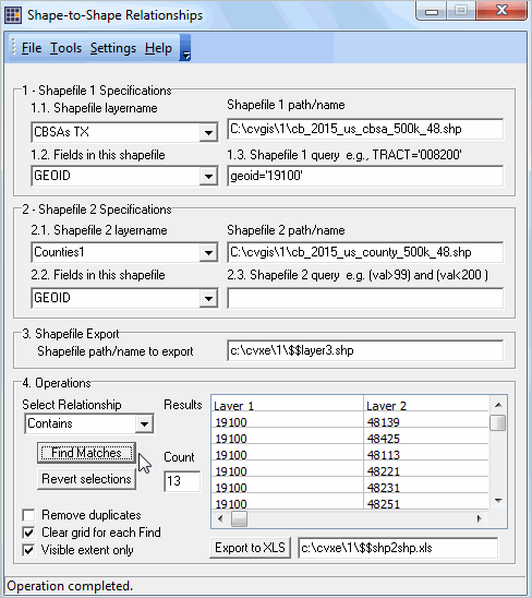 Using Touch Operation Select the type of geographic operation as Touch. Click Find Matches button. The map view now shows as:  Using Contains Operation Click RevertAll button. Select the type of geographic operation as Contains. Click Find Matches button. The map view now shows as: 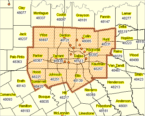 School Attendance Zones & Census Blocks -- using the resulting data The graphic shown below illustrates census blocks intersecting with Joyner Elementary School attendance zone located in Guilford County Schools, NC (see district profile). The attendance zone is shown with bold blue boundary. Joyner ES SAZ intersecting blocks are shown with black boundaries and labeled with Census 2010 total population (item P0010001 as described in table below graphic). Joyner ES is shown with red marker in lower right. The census blocks - school attendance zones were geospatially related using Shp2Shp. Geographic relationship files were developed separately for each type of zone (ES, MS, HS). The school attendance zone geocodes were then integrated into the census block shapefile for each block in the district. Click the graphic below for a larger view. Expand browser to full window for best quality view. The larger view shows a mini-profile for the census block where Joyner ES is located. The mini profile shows attributes of this block included the relevant SAZ 1 (ES), SAZ 2 (MS) and SAZ3 (HS) codes. The mini profile also shows selected Census 2010 demographics obtained using the DEDE software. A next step would be to analyze characteristics of the attendance zone based on Census 2010 demographics. The selected demographic item field names/descriptions are shown below the graphic. 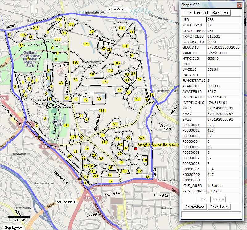 - view developed using CV XE GIS and related GIS project; click graphic for larger view Click links below to show/hide additional illustrative views • Patterns of Hispanic Population by Attendance Zone • Patterns of Hispanic Population by Attendance Zone -with Population Ages 5-17 • Patterns of Hispanic Population by Attendance Zone in Context of City Description of items shown in mini profile - scroll section
Block Items
P0010001 - Total Population P0030002 - White alone P0030003 - Black or African American alone P0030004 - American Indian and Alaska Native alone P0030005 - Asian alone P0030006 - Native Hawaiian and Other Pacific Islander alone P0030007 - Some Other Race alone P0030008 - Two or More Races P0040003 - Hispanic (of any race) H0030001 - Housing units H0030002 - Occupied H0030003 - Vacant P0140001 - Total population P0140002 - Male P0140003 - Male-Under 1 year P0140004 - Male-1 year P0140005 - Male-2 years P0140006 - Male-3 years P0140007 - Male-4 years P0140008 - Male-5 years P0140009 - Male-6 years P0140010 - Male-7 years P0140011 - Male-8 years P0140012 - Male-9 years P0140013 - Male-10 years P0140014 - Male-11 years P0140015 - Male-12 years P0140016 - Male-13 years P0140017 - Male-14 years P0140018 - Male-15 years P0140019 - Male-16 years P0140020 - Male-17 years P0140021 - Male-18 years P0140022 - Male-19 years P0140023 - Female P0140024 - Female-Under 1 year P0140025 - Female-1 year P0140026 - Female-2 years P0140027 - Female-3 years P0140028 - Female-4 years P0140029 - Female-5 years P0140030 - Female-6 years P0140031 - Female-7 years P0140032 - Female-8 years P0140033 - Female-9 years P0140034 - Female-10 years P0140035 - Female-11 years P0140036 - Female-12 years P0140037 - Female-13 years P0140038 - Female-14 years P0140039 - Female-15 years P0140040 - Female-16 years P0140041 - Female-17 years P0140042 - Female-18 years P0140043 - Female-19 years Block Group Items B02001_001E >>Total: B02001_002E >>White alone B02001_003E >>Black or African American alone B02001_004E >>American Indian and Alaska Native alone B02001_005E >>Asian alone B02001_006E >>Native Hawaiian and Other Pacific Islander alone B02001_007E >>Some other race alone B02001_008E >>Two or more races: B03002_012E Hispanic or Latino B19013_001E Median household income B25077_001E Median value (dollars) B11001_001E >>Total: B11001_002E >>Family households: B11001_003E >>Married-couple family B11001_004E >>Other family: B11001_005E >>Male householder, no wife present B11001_006E >>Female householder, no husband present B11001_007E >>Nonfamily households: B11001_008E >>Householder living alone B11001_009E >>Householder not living alone B15003_001E >>Total:E >>B15003. Educational Attainment for the Population 25 Years and OverE >>not requiredE >>int B15003_002E >>No schooling completedE >>B15003. Educational Attainment for the Population 25 Years and OverE >>not requiredE >>int B15003_003E >>Nursery schoolE >>B15003. Educational Attainment for the Population 25 Years and OverE >>not requiredE >>int B15003_004E >>KindergartenE >>B15003. Educational Attainment for the Population 25 Years and OverE >>not requiredE >>int B15003_005E >>1st gradeE >>B15003. Educational Attainment for the Population 25 Years and OverE >>not requiredE >>int B15003_006E >>2nd gradeE >>B15003. Educational Attainment for the Population 25 Years and OverE >>not requiredE >>int B15003_007E >>3rd gradeE >>B15003. Educational Attainment for the Population 25 Years and OverE >>not requiredE >>int B15003_008E >>4th gradeE >>B15003. Educational Attainment for the Population 25 Years and OverE >>not requiredE >>int B15003_009E >>5th gradeE >>B15003. Educational Attainment for the Population 25 Years and OverE >>not requiredE >>int B15003_010E >>6th gradeE >>B15003. Educational Attainment for the Population 25 Years and OverE >>not requiredE >>int B15003_011E >>7th gradeE >>B15003. Educational Attainment for the Population 25 Years and OverE >>not requiredE >>int B15003_012E >>8th gradeE >>B15003. Educational Attainment for the Population 25 Years and OverE >>not requiredE >>int B15003_013E >>9th gradeE >>B15003. Educational Attainment for the Population 25 Years and OverE >>not requiredE >>int B15003_014E >>10th gradeE >>B15003. Educational Attainment for the Population 25 Years and OverE >>not requiredE >>int B15003_015E >>11th gradeE >>B15003. Educational Attainment for the Population 25 Years and OverE >>not requiredE >>int B15003_016E >>12th grade, no diplomaE >>B15003. Educational Attainment for the Population 25 Years and OverE >>not requiredE >>int B15003_017E >>Regular high school diplomaE >>B15003. Educational Attainment for the Population 25 Years and OverE >>not requiredE >>int B15003_018E >>GED or alternative credentialE >>B15003. Educational Attainment for the Population 25 Years and OverE >>not requiredE >>int B15003_019E >>Some college, less than 1 yearE >>B15003. Educational Attainment for the Population 25 Years and OverE >>not requiredE >>int B15003_020E >>Some college, 1 or more years, no degreeE >>B15003. Educational Attainment for the Population 25 Years and OverE >>not requiredE >>int B15003_021E >>Associate's degreeE >>B15003. Educational Attainment for the Population 25 Years and OverE >>not requiredE >>int B15003_022E >>Bachelor's degreeE >>B15003. Educational Attainment for the Population 25 Years and OverE >>not requiredE >>int B15003_023E >>Master's degreeE >>B15003. Educational Attainment for the Population 25 Years and OverE >>not requiredE >>int B15003_024E >>Professional school degreeE >>B15003. Educational Attainment for the Population 25 Years and OverE >>not requiredE >>int B15003_025E >>Doctorate degreeE >>B15003. Educational Attainment for the Population 25 Years and OverE >>not requiredE >>int B25002_001E >>Total: B25002_002E >>Occupied B25002_003E >>Vacant B25003_001E >>Total: B25003_002E >>Owner occupied B25003_003E >>Renter occupied B25024_001E >>Total: B25024_002E >>1, detached B25024_003E >>1, attached B25024_004E >>2 B25024_005E >>3 or 4 B25024_006E >>5 to 9 B25024_007E >>10 to 19 B25024_008E >>20 to 49 B25024_009E >>50 or more B25024_010E >>Mobile home B25024_011E >>Boat, RV, van, etc. B01001_002E >>Male: B01001_003E >>Under 5 years B01001_004E >>5 to 9 years B01001_005E >>10 to 14 years B01001_006E >>15 to 17 years B01001_007E >>18 and 19 years B01001_008E >>20 years B01001_009E >>21 years B01001_010E >>22 to 24 years B01001_011E >>25 to 29 years B01001_012E >>30 to 34 years B01001_013E >>35 to 39 years B01001_014E >>40 to 44 years B01001_015E >>45 to 49 years B01001_016E >>50 to 54 years B01001_017E >>55 to 59 years B01001_018E >>60 and 61 years B01001_019E >>62 to 64 years B01001_020E >>65 and 66 years B01001_021E >>67 to 69 years B01001_022E >>70 to 74 years B01001_023E >>75 to 79 years B01001_024E >>80 to 84 years B01001_025E >>85 years and over B01001_026E >>Female: B01001_027E >>Under 5 years B01001_028E >>5 to 9 years B01001_029E >>10 to 14 years B01001_030E >>15 to 17 years B01001_031E >>18 and 19 years B01001_032E >>20 years B01001_033E >>21 years B01001_034E >>22 to 24 years B01001_035E >>25 to 29 years B01001_036E >>30 to 34 years B01001_037E >>35 to 39 years B01001_038E >>40 to 44 years B01001_039E >>45 to 49 years B01001_040E >>50 to 54 years B01001_041E >>55 to 59 years B01001_042E >>60 and 61 years B01001_043E >>62 to 64 years B01001_044E >>65 and 66 years B01001_045E >>67 to 69 years B01001_046E >>70 to 74 years B01001_047E >>75 to 79 years B01001_048E >>80 to 84 years B01001_049E >>85 years and over Relating Congressional Districts to Census Block Geography/Data [goto top] Shp2Shp provides unique capabilities to determine/show/analyze data/geography visually and in tabular form -- determining census blocks comprising political geography such as cities, state legislative districts and congressional districts. The following example illustrates this process using North Carolina 115th Congressional Districts and Census 2010 census blocks using TIGER 2016 shapefiles. This process can be applied to any state/sub-state area. The following graphic shows North Carolina Congressional District 13 (CD 3713) with red boundary and cross-hatch pattern. The CD intersects with five counties. The cross-hatch pattern is actually cross-hatching of census blocks contained within CD 3713. The cross-hatching was applied automatically (census block shapes selected) through use of the Shp2Shp tool. The map view shows census blocks determined to be within CD 3713 based on geospatially-determined geography. The blue cross-hatched area is Greensboro, NC. This illustrates how unrelated geography can be used for visual reference purposes. It could have been a state legislative district, census tract grouping or any other geographic area. See Shp2Shp operations section in next view. . 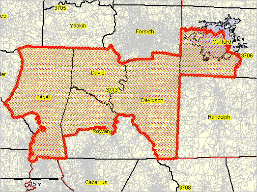 - view created using the CV XE GIS. The Shp2Shp operations form used to develop the above graphic is shown below. The controls reflect usage of "Find Matches - Contains" operations using the North Carolina CD 115 shapefile and North Carolina census blocks shapefile. A query is applied to the CD 115 shapefile to process only CD 3713. Without the query all North Carolina CDs would be processed. GEOIDs for the CDs and blocks selected/geospatially matched are shown for grid display. In addition, the census block Census 2010 total population (P0010001) is selected for display in column 3 of the grid. The grid footer shows the total number of blocks within the CD (20,432) and the sum of the block population (733,499). The process could be repeated selecting any Census 2010 block level subject matter item. A query can also be applied to the census blocks shapefile (2.3. edit box), not used in this application. Optionally check the checkbox "Visible Extent Only" to restrict match processing to a visually determined subset of the CD (not used here). The matches data shown in the grid can be optionally exported to an Excel, CSV or dBase structured file -- a congressional district Block Equivalency File. 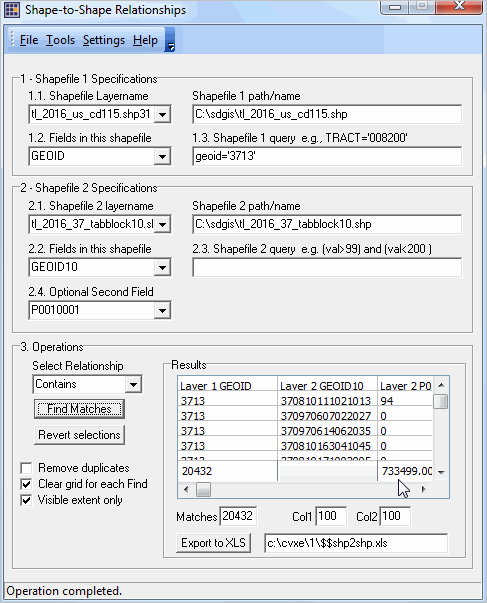 Note that 115th Congressional District Block Equivalency Files are available by state as datasets. Contact us for more information; mention "CD BEF availability" in the text section. Shp2Shp provides the ability to develop the CD BEF datasets. But in addition, Shp2Shp provides the ability: • to apply a query on the CD shapefile (include only one of a selected set of CDs) • to apply a query on the Blocks shapefile (include only blocks that meet certain geographic/demographic criteria • create a BEF with integrated subject matter data at the block level and summarized for the CD .. repeat this process to examine additional/alternative demographics • to view the data in a map optionally in context with other geography (e.g., cities/state legislative districts) .. as separate layers • to zoom-in to a neighborhood or study area of interest to view details Support Using these Resources [goto top] Learn more about demographic economic data and related analytical tools. Join us in a Data Analytics Lab session. There is no fee for these Web sessions. Each informal session is focused on a specific topic. The open structure also provides for Q&A and discussion of application issues of interest to participants. ProximityOne User Group [goto top] Join the ProximityOne User Group to keep up-to-date with new developments relating to geographic-demographic-economic decision-making information resources. Receive updates and access to tools and resources available only to members. Use this form to join the User Group. Additional Information ProximityOne develops geodemographic-economic data and analytical tools and helps organizations knit together and use diverse data in a decision-making and analytical framework. We develop custom demographic/economic estimates and projections, develop geographic and geocoded address files, and assist with impact and geospatial analyses. Wide-ranging organizations use our tools (software, data, methodologies) to analyze their own data integrated with other data. Follow ProximityOne on Twitter at www.twitter.com/proximityone. Contact us (888-364-7656) with questions about data covered in this section or to discuss custom estimates, projections or analyses for your areas of interest. |
|
|